22 Vegetation Sampling Methods, and When to Use Each

There is no single agreed count of vegetation sampling methods, because different traditions draw the boundaries in different places. This guide uses one clear rule and applies it consistently: a method counts separately when it measures a different vegetation attribute, or uses a different sampling geometry. Under that rule there are 22 methods, grouped into six families: cover, frequency, density, production, structure and remote sensing. Below you will find all 22, what each one measures, how to set it up, and the situations where it is the right call rather than the convenient one.Careful monitoring pays off. A 2025 analysis found insects declining even in pristine ecosystems, a trend only visible because researchers kept collecting standardised field data year after year. That is what these methods are for. The measurement you take this season only becomes evidence when somebody takes the same measurement in the same way for thirty years, which is why choosing the right method, and then sticking to it, matters more than choosing a clever one.

Key takeaways

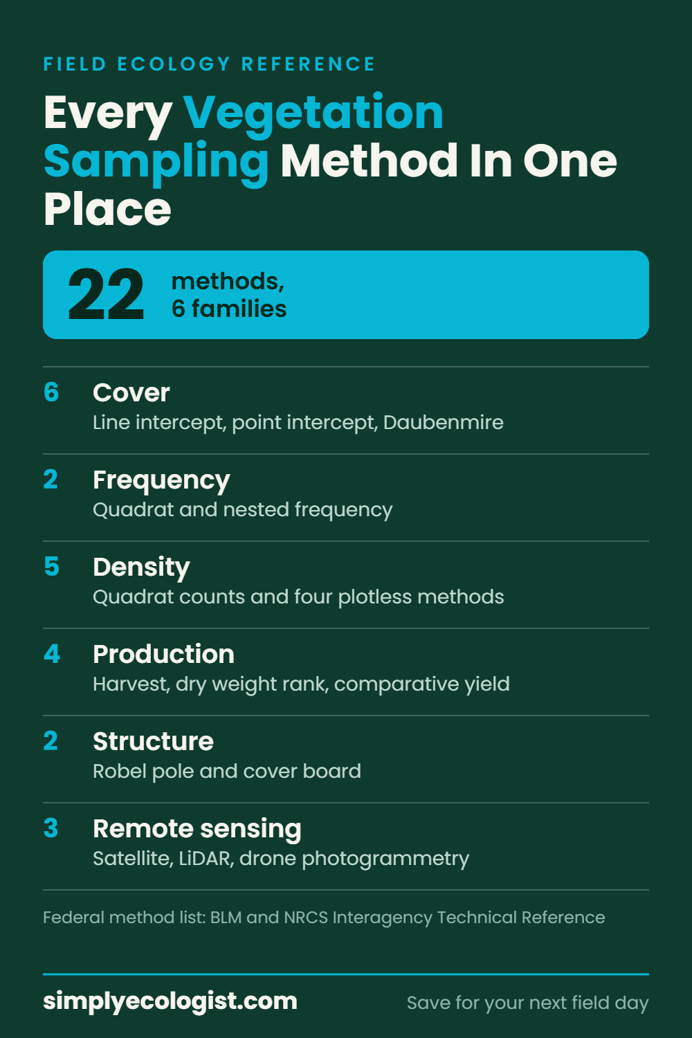
• There are 22 vegetation sampling methods in six families, counted by the attribute measured and the sampling geometry.
• Cover methods answer how much ground a species occupies. Frequency answers how often it turns up. Density answers how many there are. These three are not interchangeable.
• Plotless methods estimate density with no plots at all, which is why they beat quadrats in scattered woodland and savanna.
• The federal reference, the BLM and NRCS Interagency Technical Reference 1734 4, documents 13 of these methods in full. It predates drones, so it covers none of the remote sensing family.
• Plot size is the most common thing people get wrong. 1 m² suits herbaceous vegetation, 4 m² suits grassland composition, and forests need 100 to 400 m².

How the 22 methods are organised

Most guides organise vegetation sampling by equipment, which is why they end up describing quadrats twice. Quadrats, tapes and pins are tools. What actually distinguishes one method from another is the attribute it measures, and this is how the federal manual organises it too. Six families, and every method sits in exactly one of them.

Family	Methods	The question it answers
Cover	6	How much ground does this species occupy?
Frequency	2	How often does it turn up when I look?
Density	5	How many individuals are there per unit area?
Production	4	How much biomass is this ground growing?
Structure	2	How is the vegetation arranged vertically?
Remote sensing	3	What is happening across the whole landscape?

If you are still deciding what your survey is for rather than how to run it, start with the broader picture in this guide to designing an ecological survey, then come back here to pick the method.

Cover methods (6)

Cover is the vertical projection of plant material onto the ground, expressed as a percentage. It is the most widely reported vegetation attribute because it correlates with biomass, competitive dominance and habitat quality, and because it can be measured without counting anything. The six methods below all produce cover, but they differ in whether the observer estimates it or the equipment measures it, and that distinction is the single biggest source of disagreement between datasets.

1. Line intercept

Line intercept estimates cover by stretching a tape across the vegetation and recording the length of tape intercepted by each species canopy. Cover for a species is the total intercepted length divided by the total tape length. It is method 5 in the federal manual and it is the workhorse of shrubland and rangeland cover work.To run it, lay a tape along a randomly placed line, then walk it recording the start and end point of every canopy that crosses directly above or below the tape. Gaps within a canopy larger than a stated threshold, commonly 5 cm, are subtracted. The threshold has to be recorded, because a dataset collected with a 2 cm gap rule is not comparable to one collected with a 15 cm rule.Line intercept is at its best on vegetation with distinct, measurable canopy boundaries: shrubs, bunchgrasses, cushion plants. It is fast, it needs almost no equipment, and it is far less prone to observer disagreement than any method that asks a person to estimate a percentage by eye. Its weakness is the mirror image of its strength. On dense continuous swards where canopies overlap and boundaries are impossible to call, intercept lengths become guesswork, and on very sparse vegetation a single line may cross almost nothing, so you need many more lines than you expect.

2. Point intercept

Point intercept estimates cover by lowering a thin pin vertically at fixed intervals along a transect and recording every species the pin touches on its way to the ground. Cover is the proportion of pins that hit a given species. It is method 7 in the federal manual and the closest thing vegetation science has to an objective cover measurement.Set a transect, then lower the pin at a fixed interval, commonly every 20 to 50 cm depending on patch size. Record every contact, not just the first, because the pin passing through three layers tells you about vertical structure as well as ground cover. A pin frame holding ten pins speeds this up considerably. Sampling intensity matters more here than in any other cover method: with too few points, cover estimates for uncommon species swing wildly.The reason to choose point intercept over anything else is repeatability. A pin does not have an opinion. Two observers running the same transect will produce nearly the same numbers, which is exactly what a long term monitoring programme needs and what ocular estimation cannot deliver. It is also less destructive than harvesting and quick enough for large sample sizes.Its known weakness is rare and small leaved species. A pin is a dimensionless probe, so a plant occupying a small fraction of the ground is unlikely to be hit at all, and species present in the plot can record as zero cover. The fix is to increase point density, or to pair the transect with a presence list from a quadrat so nothing goes unrecorded.

3. Daubenmire cover class

The Daubenmire method estimates cover by placing a fixed frame, classically 20 by 50 cm, and assigning each species to a cover class rather than a precise percentage. The standard six classes are 0 to 5, 5 to 25, 25 to 50, 50 to 75, 75 to 95 and 95 to 100 percent, and the midpoint of each class is used in analysis. It is method 4 in the federal manual.Place the frame at predetermined points along a transect, then for every species rooted in or overhanging the frame, record its class. The whole point of the class system is that people are much better at agreeing which broad band a cover value falls into than at agreeing on an exact number, so binning the estimate absorbs most of the observer disagreement instead of pretending it does not exist.Daubenmire is the right choice when you need many plots quickly, in herbaceous or low vegetation, and when your analysis can live with class midpoints. It is the standard on a great deal of rangeland monitoring for exactly that reason. Its limitation is resolution. Real change inside a wide class, a species moving from 30 to 48 percent cover, is invisible in the data, and the wide middle classes are where most rangeland species sit. If your question is about gradual change, use point intercept instead.

4. Step point

Step point estimates cover by walking a route and recording what lies under a mark on the boot toe, or the tip of a pin dropped at each pace. Cover is the proportion of steps hitting each species. It is method 6 in the federal manual, and it exists because it is fast: a single observer can cover very large areas without laying a single tape. Its cost is precision and randomness, since a walked route is not a random sample and pacing introduces its own bias. Use it for broad reconnaissance across big units, not for detecting subtle change.

5. Braun-Blanquet cover abundance (releve)

The Braun-Blanquet approach records every species in a plot with a combined cover abundance score on an ordinal scale (r, +, 1, 2, 3, 4, 5), where low values blend abundance with cover and high values are cover bands. This is the backbone of the phytosociological releve tradition and of most European vegetation classification. It is fast, it captures the full species list rather than just the common ones, and decades of comparable data exist in this format. The catch is that the scale is ordinal, not interval, so cover values have to be transformed before most statistical analysis, and different transformations produce measurably different community similarity results.

6. Photo quadrat and digital image analysis

A photo quadrat records cover by photographing a fixed frame from directly above and classifying the pixels, either by hand with a point grid overlaid on the image or automatically with image analysis software. The measurement moves from the field to the desk, which means the raw data is archived permanently and can be reanalysed when your methods or questions change. It works well on low, flat vegetation with distinguishable species and poorly on anything with vertical layering, since a camera sees only the top canopy. It is also the family member that has improved fastest, because the classification step now benefits from the same machine learning that drives remote sensing.

Frequency methods (2)

Frequency is the proportion of sample units in which a species occurs. It is not abundance and it is not cover, and treating it as either is one of the most common analytical mistakes in vegetation monitoring. What frequency is very good at is detecting change cheaply, because recording presence or absence is fast, requires no estimation, and produces almost no observer disagreement.

7. Quadrat frequency

Quadrat frequency measures how often a species occurs by placing quadrats and recording, for each one, only whether the species is present. Frequency is the percentage of quadrats containing it. It is method 2 in the federal manual and the method most long term monitoring programmes are actually built on.Place quadrats at random or at systematic intervals along transects, then for each quadrat write down the species present. That is the whole field protocol, which is why a person can collect a very large sample in a day and why the numbers hold up between observers who would never agree on a cover estimate.The critical design decision is quadrat size, and it is where most frequency datasets go wrong. Frequency values are meaningless without the plot size attached, because the same population sampled at 0.1 m² and at 1 m² returns completely different frequencies. The working rule is to choose a size that puts your target species between 20 and 80 percent frequency. Below 20 percent you will not detect change without an enormous sample, and above 80 percent the species approaches every quadrat and the measure saturates, so real declines stay invisible until they are severe.Standard starting sizes are 1 m by 1 m for herbaceous vegetation and 10 m by 10 m for woody vegetation, adjusted after a pilot run. Frequency is the right method when your question is whether something is changing across a large area, when budget or time is tight, and when you need data that different field crews across different years can be trusted to have collected the same way. It is the wrong method when you need to know how much of something there is, because it will not tell you.

8. Nested frequency

Nested frequency solves the plot size problem by using several quadrat sizes at once, one inside another, commonly four nested frames. A species is recorded in the smallest frame it occurs in, which yields a frequency value at every scale from a single sample placement. Common species land in the useful 20 to 80 percent band in the small frames while rare species land in it in the large ones, so a single survey tracks both without you having to guess the right size in advance. The cost is a slightly slower field protocol and a data sheet that field crews need training to fill in correctly.

Density methods (5)

Density is the number of individuals per unit area. It is the most intuitive vegetation attribute and the hardest to measure well, for two reasons. First, you have to be able to tell what an individual is, which is straightforward for trees and close to impossible for rhizomatous grasses. Second, on sparse or clumped vegetation, plots either catch nothing or catch a clump, and both outcomes waste effort. The four plotless methods below exist entirely to solve that second problem.

9. Quadrat and belt transect counts

Plot based density counts every individual rooted inside a defined area and divide by that area. It is method 9 in the federal manual, and it is the reference standard the plotless methods are validated against.The choice is between a square or rectangular quadrat and a belt transect, which is simply a long thin quadrat defined by two parallel lines. Belt widths commonly run from 0.5 to 2 m for herbaceous and small shrub work, and wider for trees. The federal manual is explicit that long thin quadrats outperform square or circular ones of the same area for density work, because an elongated plot crosses more of the patchiness in the vegetation and therefore captures a more representative count.Plot size follows the vegetation. For herbaceous communities 1 to 4 m² is usually enough, while woody vegetation needs 100 to 400 m². The comparison of plot sizes across European vegetation by Chytry and Otypkova is the standard reference here: 4 m² captures grassland composition, 16 m² suits forest understory, and forest plots need 100 to 400 m². Sample a forest at 4 m² and you will miss most of what is standing in it.Use plot counts when individuals are countable and reasonably evenly distributed, and when you want a number you can defend without any modelling assumptions. Avoid them when the vegetation is sparse and clumped, because you will spend the day laying plots over bare ground.

10. Point centred quarter

Point centred quarter estimates density with no plots at all. At each sample point you divide the surrounding area into four quadrants with two perpendicular lines, then measure the distance from the point to the nearest qualifying individual in each quadrant. Mean distance across all measurements converts to density, because in a random distribution the mean point to plant distance carries the information a plot count would.Each point yields four distances, so twenty points give eighty measurements, and the field kit is a tape and a compass. That is the appeal: in open woodland or savanna, laying a 400 m² plot to count six trees is an hour of work for very little information, while a point centred quarter sample walks the same ground and returns density, relative density, basal area and dominance for every species encountered.The method carries an assumption that plot counts do not: it expects individuals to be randomly distributed. Real vegetation is usually clumped, and clumping biases plotless density estimates, generally downward. Simulation and field comparisons in mangrove forest have shown the size of that bias varies substantially between the plotless methods, so if your stand is strongly aggregated, either increase sample points considerably or validate against a small number of full plots.

11. Nearest neighbour (closest individual)

The closest individual method records the distance from each random sample point to the single nearest plant, and nearest neighbour records the distance from that plant to its own nearest neighbour. Both convert distance to density through the same logic as point centred quarter, with less work per point and correspondingly more sensitivity to non random spacing. They are most useful as a rapid density estimate in open vegetation, and as a diagnostic: the ratio between the two distances indicates whether a stand is clumped, random or regularly spaced.

12. Wandering quarter

The wandering quarter moves through the stand rather than sampling fixed points. From a starting individual you look forward within a defined angle, commonly 90 degrees, move to the nearest plant inside that wedge, then repeat, wandering across the stand in a chain of measured steps. It handles clumped and patchy distributions better than point based plotless methods, because the path follows the vegetation rather than landing at random on gaps. It is slower and its statistical treatment is less standardised, which is why it appears in the literature far more often than in field manuals.

13. Bitterlich variable radius (angle count)

The Bitterlich method estimates basal area per hectare by standing at a point and sweeping a fixed angle across the horizon with a wedge prism or relascope, counting every stem whose diameter appears wider than the angle. Whether a tree is counted depends on both its size and its distance, so large trees are sampled from further away and small ones only from close by. No plot is laid and no distance is measured, and one sweep gives basal area directly, which is why it is standard in forest inventory. It has also been adapted to sample basal ground cover of bunchgrasses. Its assumptions are stricter than most methods here: it needs reasonable visibility and it is not suited to dense understory.

Production and biomass methods (4)

Production methods measure how much plant material a piece of ground is growing, usually as dry weight per unit area. This family comes almost entirely from rangeland science, where the practical question is how much forage exists, and it is the family most likely to be unfamiliar to ecologists trained on cover and composition. All four sit in the federal manual.

14. Harvest (clip and weigh)

The harvest method measures production directly. You clip all the vegetation inside a plot, usually by species or functional group, dry it to constant weight, and weigh it. Everything else in this family is an estimation technique calibrated against this one, which is why it is the reference standard even though it is rarely the practical choice.The protocol is unforgiving in a useful way. Clip to a stated height, keep the material in labelled bags, dry at a stated temperature until the weight stops changing, then weigh. Field wet weight is not production, because moisture content varies enormously between species and between mornings, so the drying step is not optional. Current year growth has to be separated from older material if the question is annual production.Harvest gives you a number with no estimation and no observer bias in it, which is exactly why it anchors the other three methods. The costs are real: it is slow, it needs an oven and a balance, and it is destructive, which rules it out on permanent monitoring plots and on anything protected. The standard compromise is to harvest a small calibration subsample and estimate the rest with one of the methods below.

15. Double weight sampling

Double weight sampling is the calibration bridge. The observer estimates the weight of vegetation in a plot by eye, then actually clips and weighs a subset of those same plots. The relationship between estimated and actual weights across the clipped subset corrects every estimate in the dataset. It delivers most of the accuracy of harvesting for a fraction of the clipping, and it improves as the observer eye trains against real weights through the season. It is method 10 in the federal manual.

16. Dry weight rank

Dry weight rank records, for each plot, only which three species contribute the most dry weight, ranked first, second and third. Standard multipliers convert the accumulated ranks across many plots into species composition by weight. It is very fast, needs no scales in the field, and answers the composition question well. What it will not give you is total production, so it is normally run alongside comparative yield, which supplies the total the ranks are then applied to.

17. Comparative yield

Comparative yield estimates total production by scoring each plot against five reference plots that span the range of standing crop on the site, from lowest to highest. The observer assigns a rank of 1 to 5 rather than a weight, and a small number of clipped reference plots calibrate the ranks into actual production. Because the observer is comparing like with like on the same site on the same day, the method is fast and reasonably consistent, and it pairs with dry weight rank to give total production and species composition from the same plots.

Structure methods (2)

Structure methods measure how vegetation is arranged vertically rather than what species it contains. They matter most in wildlife work, where cover for a nesting bird is a question about visual obstruction, not about botanical composition.

18. Robel pole (visual obstruction)

The Robel pole measures visual obstruction by standing a graduated pole in the vegetation and recording, from a fixed distance and a fixed eye height, the lowest band on the pole still fully visible. A denser or taller sward obscures more of the pole. It is method 13 in the federal manual, it takes seconds per reading, and it correlates well with standing crop, which means it doubles as a rapid non destructive biomass index. It is a structural measure only: it tells you nothing about which species are producing the obstruction.

19. Cover board

A cover board is a marked board of known dimensions placed in the vegetation and viewed from a fixed distance, with the observer recording the proportion of the board obscured. It works in the same way as the Robel pole but samples a vertical plane rather than a single line, and it can be read at several heights to profile obstruction through the canopy. It is method 8 in the federal manual and is standard in habitat suitability work for birds and small mammals.

Remote sensing methods (3)

The remote sensing family covers no ground in the federal manual at all, because that document was written before this equipment was affordable. These three methods do not replace field sampling. They extend it, by letting a small number of ground measurements be extrapolated across an area no field crew could walk, and every one of them still needs ground truthing to mean anything.

20. Satellite multispectral

Multispectral satellite sensors record reflectance in several wavelength bands, and indices built from those bands, most commonly NDVI, track vegetation greenness, biomass and condition across whole landscapes. The strength is coverage and time depth: continuous archives now run back decades, so you can ask what a site looked like before your study started. The constraints are spatial resolution, which is often too coarse to separate species, cloud cover, and the fact that an index is a proxy. NDVI saturates in dense canopy, so it stops discriminating exactly where biomass is highest.

21. LiDAR canopy profiling

LiDAR measures structure directly by timing laser pulses returning from the canopy and the ground, producing canopy height, vertical profile and, through allometry, biomass estimates. It is the only method in this list that measures three dimensional vegetation structure across a landscape, which makes it the natural partner to the ground based structure methods above. It penetrates canopy well enough to return a ground surface under forest. Cost and processing complexity remain the barriers, though airborne and drone mounted systems have narrowed both considerably.

22. Drone photogrammetry (structure from motion)

Drone photogrammetry builds a three dimensional model of vegetation from many overlapping photographs taken from a drone, using structure from motion algorithms to reconstruct canopy surface and height. It delivers something close to LiDAR structural data from consumer hardware, at a resolution fine enough to resolve individual shrubs and small trees.A survey means flying a planned grid with high image overlap, commonly 70 to 80 percent, then processing the images into a point cloud and a canopy height model. Ground control points measured with survey grade GPS anchor the model. In practice most of the work is the processing and the ground truthing, not the flying, and this is the step people consistently underestimate when planning a first drone survey.Two conditions matter more than most guidance admits. Reconstructed canopy heights are sensitive to wind, because a moving canopy is a moving target between overlapping frames, while they are relatively insensitive to illumination conditions, so an overcast day is not the problem people assume. Choice of processing software also measurably affects the output, which means the software version belongs in your methods section alongside the flight parameters.Use it when you need structure at fine resolution over tens of hectares, when repeat surveys will track change, or when the terrain makes ground survey impractical. Do not use it as a substitute for species level data, because a canopy surface model does not know what it is looking at. Pair it with ground plots and the combination is stronger than either alone.

Which vegetation sampling method should you use?

The honest answer is that the method follows the question, not the habitat and certainly not the equipment you happen to own. This table is the short version of everything above.

If your question is	Use	Because
Is this species increasing or declining across a large area?	Quadrat frequency	Cheapest reliable change detection, and different crews collect it consistently
How much ground does each species cover, precisely?	Point intercept	Objective, repeatable, minimal observer disagreement
How much cover, across many plots, quickly?	Daubenmire cover class	Fast, and binning absorbs observer disagreement
Cover in shrubland with clear canopy edges?	Line intercept	Measures canopy directly, needs only a tape
Full species list for community classification?	Braun-Blanquet releve	Captures rare species and matches decades of comparable data
How many trees per hectare in open woodland?	Point centred quarter	No plots to lay on ground that is mostly gaps
Basal area in forest inventory?	Bitterlich angle count	One sweep gives basal area with no plot and no distances
How much forage is this paddock growing?	Comparative yield with dry weight rank	Total production and composition from the same plots
Is there enough cover for ground nesting birds?	Robel pole	Measures visual obstruction, which is the actual habitat variable
Canopy structure across 50 hectares?	Drone photogrammetry	Fine resolution structure without walking the ground
Has greenness changed here since 1990?	Satellite multispectral	Only method with a multi decade archive

Two rules sit behind all of it. Match the attribute to the question, because cover, frequency and density are not substitutes for one another. And once you have chosen, do not change, since a monitoring dataset is only worth what its consistency is worth. If you are setting up a programme that has to run for years, the design decisions matter more than the method choice, and these biodiversity monitoring protocols cover that groundwork.

The federal reference: 13 methods in one manual

If you want a single authoritative source, the Interagency Technical Reference 1734 4, Sampling Vegetation Attributes, published jointly by the BLM, NRCS, US Forest Service and USGS, documents 13 of these methods in full, with field forms and worked calculations. It is free, it is thorough, and it is the document US agency ecologists actually work from. It contains no remote sensing and no plotless methods, which is why this guide covers 22 rather than 13.

Method	Attribute	Page
Photographs	Documentation	31
Frequency Methods	Frequency	37
Dry Weight Rank	Production	50
Daubenmire	Cover	55
Line Intercept	Cover	64
Step Point	Cover	70
Point Intercept	Cover	78
Cover Board	Cover and structure	86
Density	Density	94
Double Weight Sampling	Production	102
Harvest	Production	112
Comparative Yield	Production	116
Visual Obstruction (Robel Pole)	Structure	123

What you need in the field

Most of these methods need surprisingly little. The kit below covers the majority of them, and nothing on it is expensive except the last item.

• Quadrat frame. A 1 m by 1 m folding or sectional frame covers herbaceous work. A 20 by 50 cm Daubenmire frame covers cover class work. Sectional frames matter more than you expect, because a rigid 1 m frame is awkward to carry through dense scrub.
• Measuring tapes. Two 30 m or 50 m fibreglass tapes, one for the transect and one for perpendicular measurements. Fibreglass rather than steel, because steel tapes are heavy and take a set.
• Pin frame or a single pin. A ten pin frame turns point intercept from slow to fast. A single thin rod works and costs nothing.
• Compass and GPS. Needed for transect bearings and for relocating permanent plots. Plot relocation failure is the commonest reason long term datasets break.
• Robel pole. A graduated pole, easy to make yourself, plus a fixed length cord to standardise viewing distance.
• Wedge prism or relascope. Only if you are doing basal area work, but nothing else substitutes for it.
• Clippers, paper bags and a drying oven. For harvest and double weight sampling. A domestic oven on its lowest setting works for small samples.
• Waterproof notebook and pencil. Pencil, not pen. Every field ecologist learns this once.
• Camera. For photo quadrats and for the photographic record that is method 1 in the federal manual.
• Drone. Only for the last family, and the flying is the cheap part. Budget for processing software and for the ground control you will need to make the output mean anything.

Frequently asked questions

How many vegetation sampling methods are there?

There is no universally agreed count, because the boundary between a method and a variant is a judgement call. Counting a method separately when it measures a different attribute or uses a different sampling geometry gives 22 methods in six families. The BLM and NRCS Interagency Technical Reference documents 13 of them, omitting remote sensing and plotless methods entirely.

How many quadrats do I need?

Enough that adding more stops changing your answer. In practice, run a pilot, plot cumulative species against number of quadrats, and sample until that species area curve flattens. For frequency work there is a second target: choose a quadrat size that puts your species of interest between 20 and 80 percent frequency, because outside that band the measure cannot detect change.

What size quadrat should I use?

1 m by 1 m for herbaceous vegetation and 10 m by 10 m for woody vegetation are the standard starting points. For community composition, 4 m² captures grassland, 16 m² suits forest understory, and forest plots need 100 to 400 m². Always run a pilot rather than trusting the default, and always record the size, because frequency and cover values are meaningless without it.

Line intercept or point intercept?

Line intercept when canopies have measurable edges, as in shrubland, because you are measuring real canopy length. Point intercept when you need repeatability across observers and years, or when you also want vertical structure from multiple pin contacts. Point intercept is more objective. Line intercept is faster on sparse shrubs.

What is a plotless method and when is it better?

A plotless method estimates density from distances between a sample point and the nearest plants rather than from counts inside a defined area. It is better when vegetation is sparse or scattered, such as open woodland and savanna, where laying a plot large enough to contain individuals is slow and mostly encloses bare ground. It is worse when vegetation is strongly clumped, because the mathematics assumes something closer to a random distribution.

Can a drone replace field sampling?

No, and treating it as a replacement is the commonest mistake in a first drone survey. Photogrammetry and LiDAR measure structure, not identity. A canopy height model cannot tell you which species it is looking at, and every remote sensing output needs ground plots to calibrate and validate it. What a drone genuinely replaces is the impossible field survey, the one across ground you could never walk at that resolution.

How do I reduce observer bias?

Choose methods that measure rather than estimate. Point intercept, line intercept and frequency all leave the observer very little to judge. Where estimation is unavoidable, use classes rather than exact percentages, as Daubenmire does, and calibrate the whole crew against the same plots at the start of every season. Record the decision rules, such as the canopy gap threshold, because undocumented rules are where between year comparability quietly disappears.

Where to go next

Pick the attribute your question needs, pick the method in that family that fits your vegetation, then run a pilot before committing a season to it. Almost every disappointing vegetation dataset comes from one of two decisions: measuring the wrong attribute, or changing the method partway through. Neither is a fieldwork problem. Both are decisions made at a desk before anyone puts a frame on the ground.

Related reading: 10 Best Insect Repellents for Wildlife Research

Vegetation work sits alongside a wide range of other field techniques. If you are planning a mixed survey season, this list of ecological survey methods covers plants, habitats and every animal group in one place.